5.5 Additional examples

5.5.1 The Uniform Distribution

Another common continuous distribution is called the uniform distribution. In a uniform distribution, every value between min and max is equally likely.

We can sample from the uniform distribution using the runif() function. It takes three arguments:

• n: how many data points we want to sample
• min: the smallest possible value (default = 0)
• max: the largest possible value (default = 1)

runif(n = 5, min = -1, max = 2)

## [1] -0.07211769 -0.54521765 -0.56228067  0.16996795  1.29586515

As above, since the uniform distribution is continuous, we use a histogram to see the shape of the data. We sample 10000 data points from this min = -1, max = 2 uniform distribution:

data = runif(n = 10000, min = -1, max = 2)
hist(data, xlim = c(-2, 3), main = "Histogram of Unif(min = -1, max = 2)")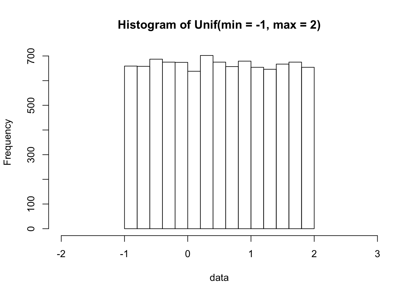

Its PDF is very simple:

curve(dunif(x, min = -1, max = 2), xlim = c(-2, 3),
      main = "PDF of Unif(min = -1, max = 2)", ylab = "Density")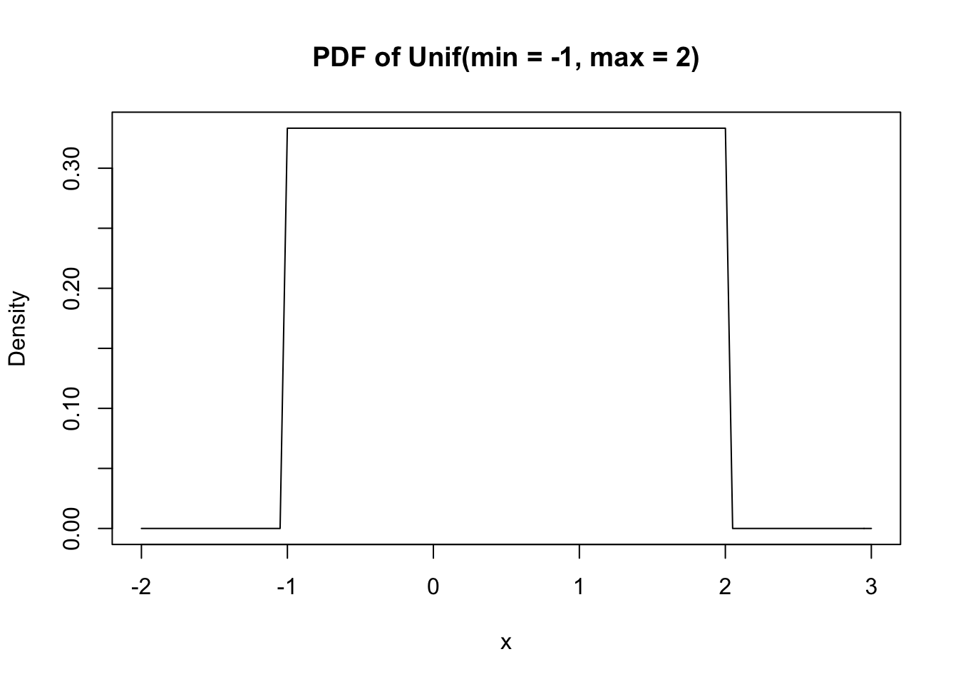

Its CDF is almost as simple:

curve(punif(x, min = -1, max = 2), xlim = c(-2, 3),
      main = "CDF of Unif(min = -1, max = 2)", ylab = "Probability")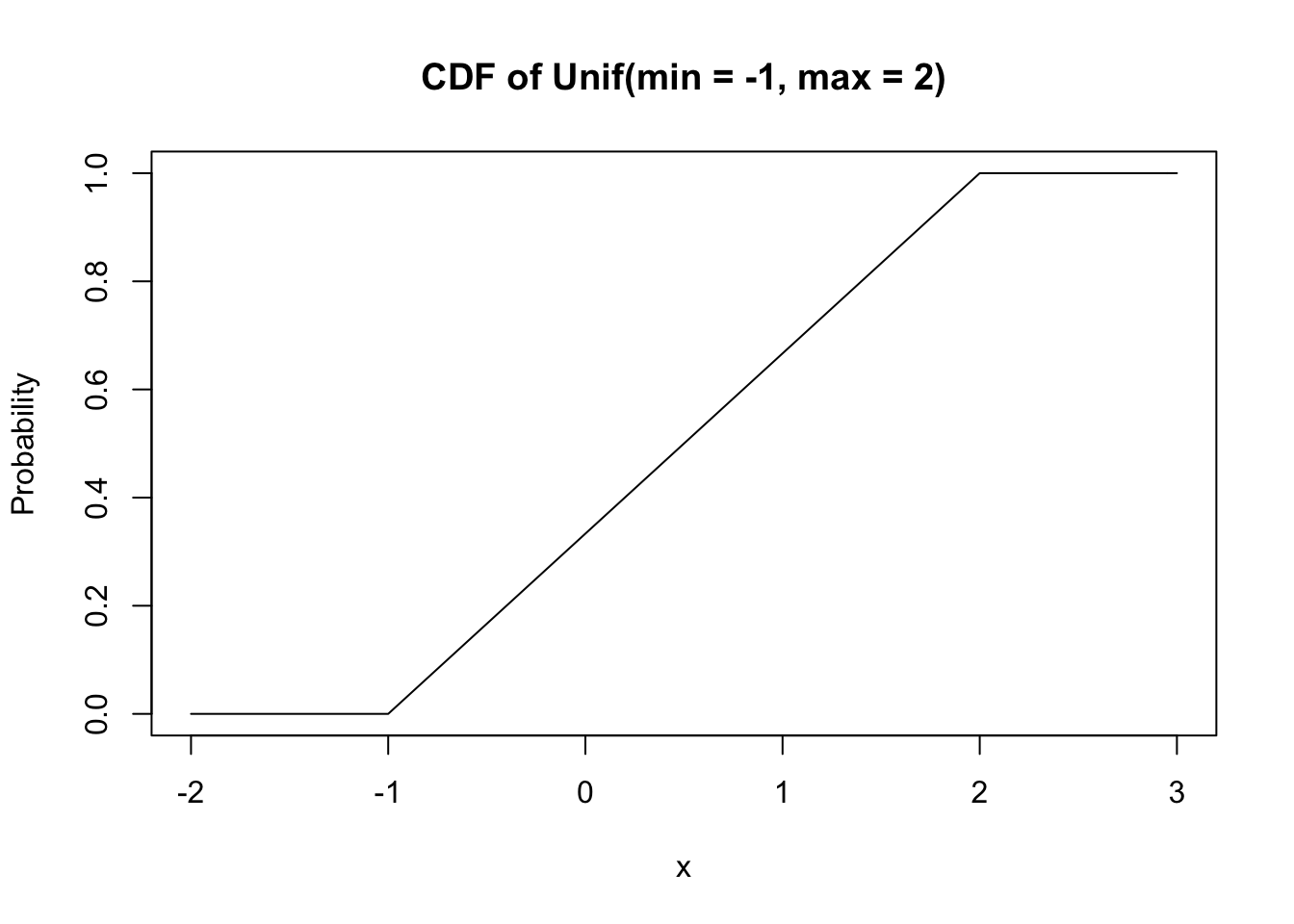

Don’t let the simplicity of the uniform fool you: it’s very important. In fact, chances are that any time you simulate from any distribution (including all of the examples in this chapter), the uniform is somehow involved under the hood!