6.2 Hypothesis Tests
6.2.1 Illustrating a Hypothesis Test
Let’s say we have a batch of chocolate bars, and we’re not sure if they are from Theo’s. What can the weight of these bars tell us about the probability that these are Theo’s chocolate?
set.seed(20)
choc.batch <- rnorm(20, mean = 42, sd = 2)
summary(choc.batch)
## Min. 1st Qu. Median Mean 3rd Qu. Max.
## 36.22 40.81 41.41 41.62 42.87 45.57Now, let’s perform a hypothesis test on this chocolate of an unknown origin.
What is the sampling distribution of the bar weight under the null hypothesis that the bars from Theo’s weigh 40 grams on average? We’ll need to specify the standard deviation to obtain the sampling distribution, and here we’ll use \(\sigma_X = 2\) (since that’s the value we used for the distribution we sampled from).
The null hypothesis is \[H_0: \mu = 40\] since we know the mean weight of Theo’s chocolate bars is 40 grams.
The sample distribution of the sample mean is: \[ \overline{X} \sim {\cal N}\left(\mu, \frac{\sigma}{\sqrt{n}}\right) = {\cal N}\left(40, \frac{2}{\sqrt{20}}\right). \] We can visualize the situation by plotting the p.d.f. of the sampling distribution under \(H_0\) along with the location of our observed sample mean.
mu.0 <- 40
sigma.0 <- 2
n <- length(choc.batch)
x.bar <- mean(choc.batch)

curve(dnorm(x, mean = mu.0, sd = sigma.0/sqrt(n)), xlim = c(38, 42),
      main = "Distribution of Chocolate Weight Under Null Hypothesis",
      xlab = "Chocolate Bar Weight (in g)", ylab = "Density", col = "blue")
abline(v = mean(choc.batch), lwd = 2)
text("Unknown batch mean", x = mean(choc.batch), y = 0.6, cex = 0.8, pos = 2)
text("Sampling distribution", x = mu.0, y = 0.3, cex = 0.8, col = "blue")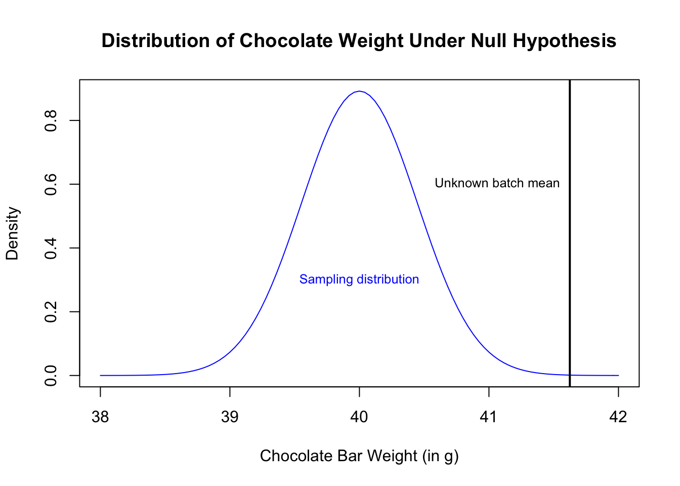
6.2.2 Hypothesis Tests for Means
6.2.2.1 Known Standard Deviation
It is simple to calculate a hypothesis test in R (in fact, we already implicitly did this in the previous section). When we know the population standard deviation, we use a hypothesis test based on the standard normal, known as a \(z\)-test. Here, let’s assume \(\sigma_X = 2\) (because that is the standard deviation of the distribution we simulated from above) and specify the alternative hypothesis to be \[
H_A: \mu \neq 40.
\] We will the z.test() function from the BSDA package, specifying the confidence level via conf.level, which is \(1 - \alpha = 1 - 0.05 = 0.95\), for our test:
library(BSDA)
zTest <- z.test(x = choc.batch, mu = 40, sigma.x = 2, conf.level = 0.95)
zTest$p.value
## [1] 0.00028076446.2.2.2 Unknown Standard Deviation
If we do not know the population standard deviation, we typically use the t.test() function included in base R. We know that: \[\frac{\overline{X} - \mu}{\frac{s_x}{\sqrt{n}}} \sim t_{n-1},\] where \(t_{n-1}\) denotes Student’s \(t\) distribution with \(n - 1\) degrees of freedom. We only need to supply the confidence level here:
tTest <- t.test(x = choc.batch, mu = 40, conf.level = 0.95)
tTest$p.value
## [1] 0.003109143We note that the \(p\)-value here (rounded to 4 decimal places) is 0.0031, so again, we can detect it’s not likely that these bars are from Theo’s. Even with a very small sample, the difference is large enough (and the standard deviation small enough) that the \(t\)-test can detect it.
6.2.3 Two-sample Tests
6.2.3.1 Unpooled Two-sample t-test
Now suppose we have two batches of chocolate bars, one of size 40 and one of size 45. We want to test whether they come from the same factory. However we have no information about the distributions of the chocolate bars. Therefore, we cannot conduct a one sample t-test like above as that would require some knowledge about \(\mu_0\), the population mean of chocolate bars.
We will generate the samples from normal distribution with mean 45 and 47 respectively. However, let’s assume we do not know this information. The population standard deviation of the distributions we are sampling from are both 2, but we will assume we do not know that either. Let us denote the unknown true population means by \(\mu_1\) and \(\mu_2\).
batch.1 <- rnorm(n = 40, mean = 45, sd = 2)
batch.2 <- rnorm(n = 45, mean = 47, sd = 2)
boxplot(batch.1, batch.2, border=c("blue","black"),
        main="Boxplot for chocolate bars from two batches",
        names=c("Batch 1","Batch 2"), ylab="Chocolate bar weight")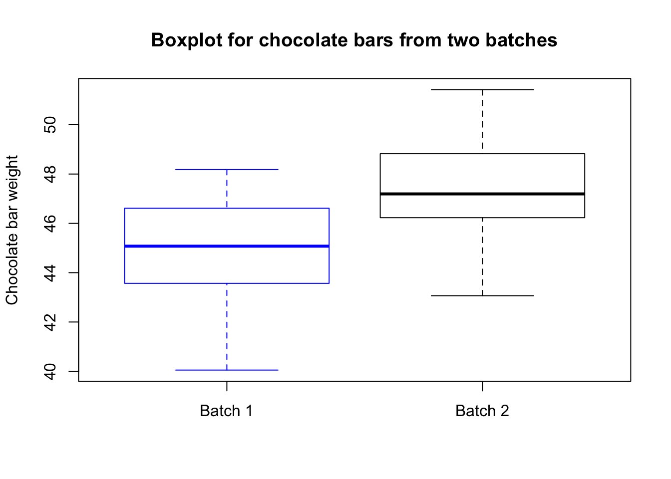
Consider the test \(H_0:\mu_1=\mu_2\) versus \(H_1:\mu_1\neq\mu_2\). We can use R function t.test again, since this function can perform one- and two-sided tests. In fact, t.test assumes a two-sided test by default, so we do not have to specify that here.
t.test(batch.1, batch.2)##
## Welch Two Sample t-test
##
## data: batch.1 and batch.2
## t = -5.658, df = 80.33, p-value = 2.278e-07
## alternative hypothesis: true difference in means is not equal to 0
## 95 percent confidence interval:
## -3.197527 -1.533586
## sample estimates:
## mean of x mean of y
## 44.98055 47.34611The p-value is much less than .05, so we can quite confidently reject the null hypothesis. Indeed, we know from simulating the data that \(\mu_1\neq\mu_2\), so our test led us to the correct conclusion!
Consider instead testing \(H_0:\mu_1=\mu_2\) versus \(H_1:\mu_1\leq\mu_2\).
t.test(batch.1, batch.2, alternative="less")##
## Welch Two Sample t-test
##
## data: batch.1 and batch.2
## t = -5.658, df = 80.33, p-value = 1.139e-07
## alternative hypothesis: true difference in means is less than 0
## 95 percent confidence interval:
## -Inf -1.669838
## sample estimates:
## mean of x mean of y
## 44.98055 47.34611As we would expect, this test also rejects the null hypothesis. One-sided tests are more common in practice as they provide a more principled description of the relationship between the datasets. For example, if you are comparing your new drug’s performance to a “gold standard”, you really only care if your drug’s performance is “better” (a one-sided alternative), and not that your drug’s performance is merely “different” (a two-sided alternative).
6.2.3.2 Pooled Two-sample t-test
Suppose you knew that the samples are coming from distributions with same standard deviations. Then it makes sense to carry out a pooled 2 sample t-test. You specify this in the t.test function as follows.
t.test(batch.1, batch.2, var.equal = TRUE)##
## Two Sample t-test
##
## data: batch.1 and batch.2
## t = -5.6794, df = 83, p-value = 1.941e-07
## alternative hypothesis: true difference in means is not equal to 0
## 95 percent confidence interval:
## -3.193986 -1.537127
## sample estimates:
## mean of x mean of y
## 44.98055 47.346116.2.3.3 Paired t-test
Suppose we take a batch of chocolate bars and stamp the Theo’s logo on them. We want to know if the stamping process significantly changes the weight of the chocolate bars. Let’s suppose that the true change in weight is distributed as a \({\cal N}(-0.3, 0.2^2)\) random variable:
choc.after <- choc.batch + rnorm(n = 20, mean = -0.3, sd = 0.2)par(mfrow = c(1,2))
boxplot(choc.batch, choc.after, border=c("blue","black"),
main="Boxplot for before and after",
names=c("Before","After"), ylab="Chocolate bar weight")
boxplot(choc.after - choc.batch, main="Boxplot for weight difference")
abline(h = 0, lty = 3, col = rgb(0, 0, 0, 0.5))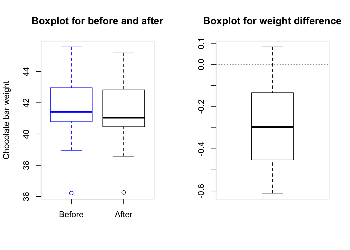
Let \(\mu_1\) and \(\mu_2\) be the true means of the distributions of chocolate weights before and after the stamping process. Suppose we want to test \(H_0:\mu_1=\mu_2\) versus \(\mu_1\neq\mu_2\). We can use the R function t.test() for this by choosing paired = TRUE, which indicates that we are looking at pairs of observations corresponding to the same experimental subject and testing whether or not the difference in distribution means is zero.
t.test(choc.after, choc.batch, paired = TRUE)##
## Paired t-test
##
## data: choc.after and choc.batch
## t = -5.9034, df = 19, p-value = 1.103e-05
## alternative hypothesis: true difference in means is not equal to 0
## 95 percent confidence interval:
## -0.3838959 -0.1829305
## sample estimates:
## mean of the differences
## -0.2834132We can also perform the same test as a one sample t-test using choc.after - choc.batch.
t.test(choc.after - choc.batch)##
## One Sample t-test
##
## data: choc.after - choc.batch
## t = -5.9034, df = 19, p-value = 1.103e-05
## alternative hypothesis: true mean is not equal to 0
## 95 percent confidence interval:
## -0.3838959 -0.1829305
## sample estimates:
## mean of x
## -0.2834132Notice that we get the exact same \(p\)-value for these two tests.
Since the p-value is less than .05, we reject the null hypothesis at level .05. Hence, we have enough evidence in the data to claim that stamping a chocolate bar significantly reduces its weight.
6.2.4 Tests for Proportions
Let’s look at the proportion of Theo’s chocolate bars with a weight exceeding 38g:
table(choc > 38) / length(choc)##
## FALSE TRUE
## 0.1607 0.8393Going back to that first batch of 20 chocolate bars of unknown origin, let’s see if we can test whether they’re from Theo’s based on the proportion weighing > 38g.
table(choc.batch > 38) / length(choc.batch)##
## FALSE TRUE
## 0.05 0.95count.unknown <- sum(choc.batch > 38)
count.unknown## [1] 19Recall from our test on the means that we rejected the null hypothesis that the means from the two batches were equal. In this case, a one-sided test is appropiate, and our hypothesis is:
Null hypothesis: \(H_0: p = 0.85\).
Alternative: \(H_A: p > 0.85\).
We want to test this hypothesis at a level \(\alpha = 0.05\).
In R, there is a function called prop.test() that you can use to perform tests for proportions. Note that prop.test() only gives you an approximate result.
prop.test(count.unknown, length(choc.batch), p = 0.85, alternative = "greater")## Warning in prop.test(count.unknown, length(choc.batch), p = 0.85,
## alternative = "greater"): Chi-squared approximation may be incorrect##
## 1-sample proportions test with continuity correction
##
## data: count.unknown out of length(choc.batch), null probability 0.85
## X-squared = 0.88235, df = 1, p-value = 0.1738
## alternative hypothesis: true p is greater than 0.85
## 95 percent confidence interval:
## 0.7702849 1.0000000
## sample estimates:
## p
## 0.95Similarly, you can use the binom.test() function for an exact result.
binom.test(count.unknown, length(choc.batch), p = 0.85, alternative = "greater")##
## Exact binomial test
##
## data: count.unknown and length(choc.batch)
## number of successes = 19, number of trials = 20, p-value = 0.1756
## alternative hypothesis: true probability of success is greater than 0.85
## 95 percent confidence interval:
## 0.7838938 1.0000000
## sample estimates:
## probability of success
## 0.95The \(p\)-value for both tests is around 0.18, which is much greater than 0.05. So, we cannot reject the hypothesis that the unknown bars come from Theo’s. This is not because the tests are less accurate than the ones we ran before, but because we are testing a less sensitive measure: the proportion weighing > 38 grams, rather than the mean weights. Also, note that this doesn’t mean that we can conclude that these bars do come from Theo’s – why not?
The prop.test() function is the more versatile function in that it can deal with contingency tables, larger number of groups, etc. The binom.test() function gives you exact results, but you can only apply it to one-sample questions.
6.2.5 Power
Let’s think about when we reject the null hypothesis. We would reject the null hypothesis if we observe data with too small of a \(p\)-value. We can calculate the critical value where we would reject the null if we were to observe data that would lead to a more extreme value.
Suppose we take a sample of chocolate bars of size n = 20, and our null hypothesis is that the bars come from Theo’s (\(H_0\): mean = 40, sd = 2). Then for a one-sided test (versus larger alternatives), we can calculate the critical value by using the quantile function in R, specifiying the mean and sd of the sampling distribution of \(\overline X\) under \(H_0\):
mu.0 <- 40
alpha <- 0.05
n <- 20
stddev <- 2

zcrit <- qnorm(1 - alpha, mean = mu.0, sd = stddev / sqrt(n))
zcrit
## [1] 40.7356Now suppose we want to calculate the power of our hypothesis test: the probability of rejecting the null hypothesis when the null hypothesis is false. In order to do so, we need to compare the null to a specific alternative, so we choose \(H_A\): mean = 42, sd = 2. Then the probability that we reject the null under this specific alternative is
mu.a <- 42

1 - pnorm(zcrit, mean = mu.a, sd = stddev / sqrt(n))
## [1] 0.9976528We can use R to perform the same calculations using the power.z.test from the asbio package:
power.test <- asbio::power.z.test(n = n, effect = mu.a - mu.0, sigma = stddev,
                    alpha = alpha, test = "one.tail")
power.test$power
## [1] 0.9976528