5.1 Simulating Random Variables for Individual Events

5.1.1 Flipping Coins

R has many functions for simulating random variables. Suppose we want to simulate a single fair coin toss (precisely defined, we want “heads” half of the time, and “tails” the other half of the time). We can use the sample() function to accomplish this, with the following code:

sample(c("heads", "tails"), size = 1)

## [1] "tails"

Now suppose we want to toss a fair coin multiple times. We can change the size arguments to achieve this (as always, you can use ? or help() to check the documentation at any time).

sample(c("heads", "tails"), size = 5, replace = TRUE)

## [1] "tails" "tails" "tails" "heads" "heads"

Note that we set replace = TRUE, which means after we get an outcome, let’s say heads, in the first toss, we will replace it back to the sample space, then do the second toss. On the contrary, if replace = FALSE, we will take heads out after the first toss, then the sample space will be {tails} when we do the second toss (and further tosses wouldn’t be possible, since we’ve exhausted all of the outcomes!)

What if we want an unfair coin? We can do that too–this code will flip a coin with a 90% chance of coming up heads:

sample(c("heads", "tails"), size = 5, replace = TRUE, prob = c(0.9, 0.1))

## [1] "heads" "heads" "heads" "tails" "heads"

In general, each element of the first input vector is matched to a corresponding probability of occurrence in the prob vector.

5.1.2 Rolling Dice

Now consider a six-sided die (plural dice). If it is a fair die, each side (labeled 1 through 6, inclusive) will have equal probability (1/6) of coming up. Its sample space is \(\{1,2,3,4,5,6\}\), but this is not a binomial random variable, since it’s only a single event rather than the sum of several events. In fact, it has a Multinoulli distribution. We can simulate this with sample() too.

sample(1:6, size = 1)

## [1] 1

As above, we can also simulate rolling multiple dice. Here we roll three six-sided dice:

sample(1:6, size = 3, replace = TRUE)

## [1] 5 1 3

We can also roll unfair dice. Here 6 should come up very often:

sample(1:6, size = 12, replace = TRUE,
       prob = c(1/10, 1/10, 1/10, 1/10, 1/10, 5/10))

##  [1] 6 6 6 6 1 6 6 1 5 4 6 4

5.1.3 Plotting Results

If we want to flip a lot of coins or roll a lot of dice, it quickly becomes impractical to go through all the results by hand. One of the best ways to explore lots of data is to plot it in some way.

Suppose we flipped a coin 20 times and want to see the results. We can use code from above and from previous tutorials to summarize the data.

data <- sample(c("heads", "tails"), size = 20, replace = TRUE)
barplot(table(data))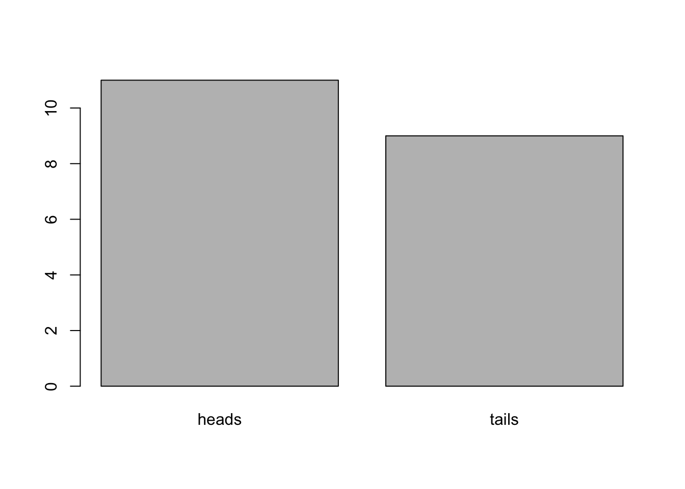

Now suppose we want to roll our unfair die 100 times.

data <- sample(1:6, size = 100, replace = TRUE,
               prob = c(1/10, 1/10, 1/10, 1/10, 1/10, 5/10))
barplot(table(data))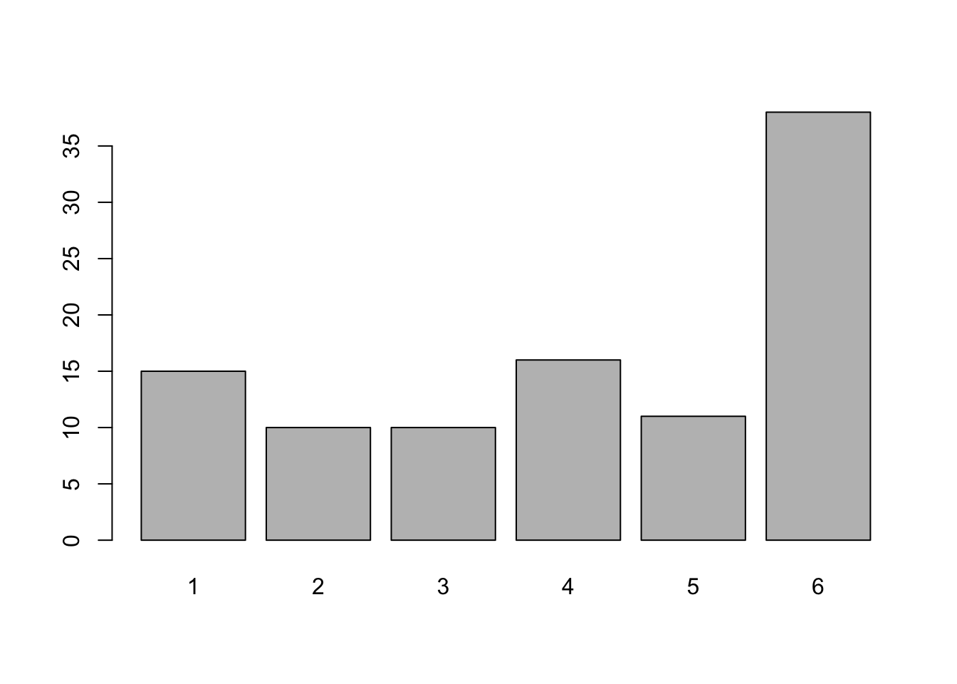

We can easily see which side is more likely to come up.