5.2 Discrete Distributions
Discrete random variables can only take values in a specified finite or countable sample space, that is, elements in it can be indexed by integers (for example, \(\{a_1,a_2,a_3,\ldots\}\)). Here we explore a couple of the most common kinds of discrete distributions. We will not (yet) go into why the distributions are the way they are, only what they look like, and how to sample data from them.
For each distribution, there are four functions.
The random sample function: when the function begins with
r, it generates (pseudo)random samples from the specified distribution. We used this in the very first lab withrnorm().The density function: when the function begins with
d, it calculates the probability (density) of a particular outcome. It is also known as the probability density function or PDF.The cumulative probability function: when the function begins with
p, it calculates the probability of a range of outcomes. It is also known as the cumulative distribution function or CDF.The quantile function: when the function begins with
q, it calculates the range of outcomes required to add up to a particular probability. It is also known as the inverse CDF.
The starting letter of the functions names for PDF and CDF can be kind of confusing. Here is an easy way to distinguish them: d for density and p for cumulative probability.
5.2.1 The Bernoulli Distribution
A Bernoulli random variable (\(X \sim \text{Bernoulli}(p)\)) is equivalent to a (not necessarily fair) coin flip, but the outcome sample space is \(\{0,1\}\) instead of heads and tails. The parameter \(p\), by convention, signifies the probability of getting a 1, and a single draw of a Bernoulli random variable is called a “trial.”
5.2.1.1 Random Samples: rbinom
The best way to simulate a Bernoulli random variable in R is to use the binomial functions (more on the binomial below), because the Bernoulli is a special case of the binomial: when the sample size (number of trials) is equal to one (size = 1).
The rbinom function takes three arguments:
n: how many observations we want to drawsize: the number of trials in the sample for each observation (here = 1)p: the probability of success on each trial
rbinom(n = 1, size = 1, p = 0.7)## [1] 1We can also randomly draw a whole bunch of Bernoulli (single) trials:
rbinom(n = 20, size = 1, p = 0.7)## [1] 0 1 1 1 0 0 1 1 0 1 0 1 1 1 1 1 0 0 1 1Check out the help function for rbinom to see the arguments you can use with this function, and their meaning.
5.2.1.2 Density Functions: dbinom
The Bernoulli has a very simple PDF, \[\Pr(X = x) = \begin{cases} p & x = 1 \\ 1 - p & x = 0 \end{cases}.\] This time, we’ll use the density function inside a barplot command, to send it directly to a plot.
barplot(names.arg = 0:1,
        height = dbinom(0:1, size = 1, p = 0.7),
        main = "Bernoulli PDF", xlab = 'X', ylab = 'Probability')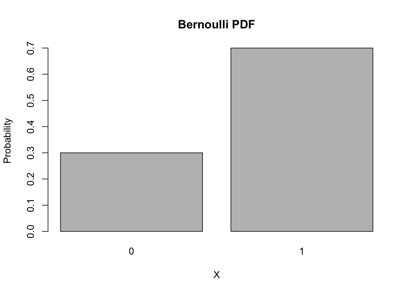
5.2.1.3 Cumulative Distribution Functions: pbinom
The CDF of a Bernoulli random variable is also simple.
barplot(names.arg = 0:1,
        height = pbinom(0:1, size = 1, p = 0.7),
        main = "Bernoulli CDF", xlab = 'X', ylab = 'Probability')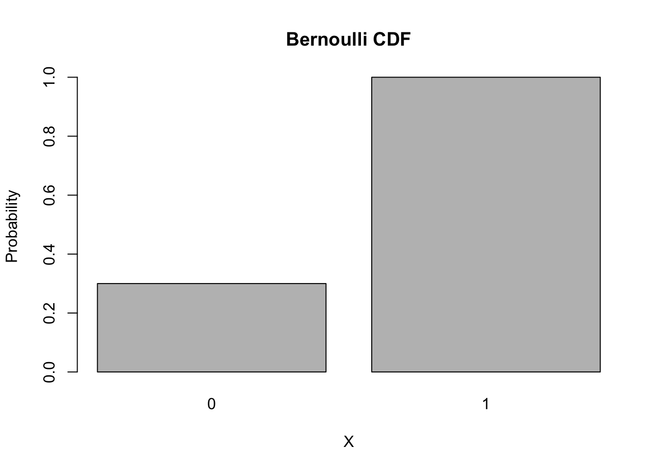
5.2.2 The Binomial Distribution
The binomial random variable is defined as the sum of repeated Bernoulli trials, so it represents the count of the number of successes (outcome=1) in a sample of these trials. The argument size in the binom functions tells R the number of Bernoulli trials we want in the sample.
5.2.2.1 Random Samples: rbinom
Notice we used the binom functions with size = 1 to explore the Bernoulli distribution above, so we just need to change this argument to sample from a binomial distribution:
rbinom(n = 15, size = 20, p = 0.7)## [1] 14 13 17 12 16 14 18 11 11 14 13 14 17 14 15This represents the process of taking 15 samples, each with 20 trials, where the probability of success in each trial is 0.7, and the outcomes are the number of successes in each sample.
Note: In the traditional notation for the binomial PDF B(n,p), we write: \[P(X=k; n,p) = {n \choose k} (p)^x (1-p)^{n-k}\] In this context \(n\) refers to the number of (bernoulli) trials in the sample.
But in R, size is used to refer to the number of trials in the sample, and n is is instead used to refer to the number of outcomes you want to randomly draw from the binomial distribution.
We can plot these outcomes if we simulate too many to examine directly,
dat <- rbinom(n = 1000, size = 20, p = 0.7)
barplot(table(dat), ylab = "counts")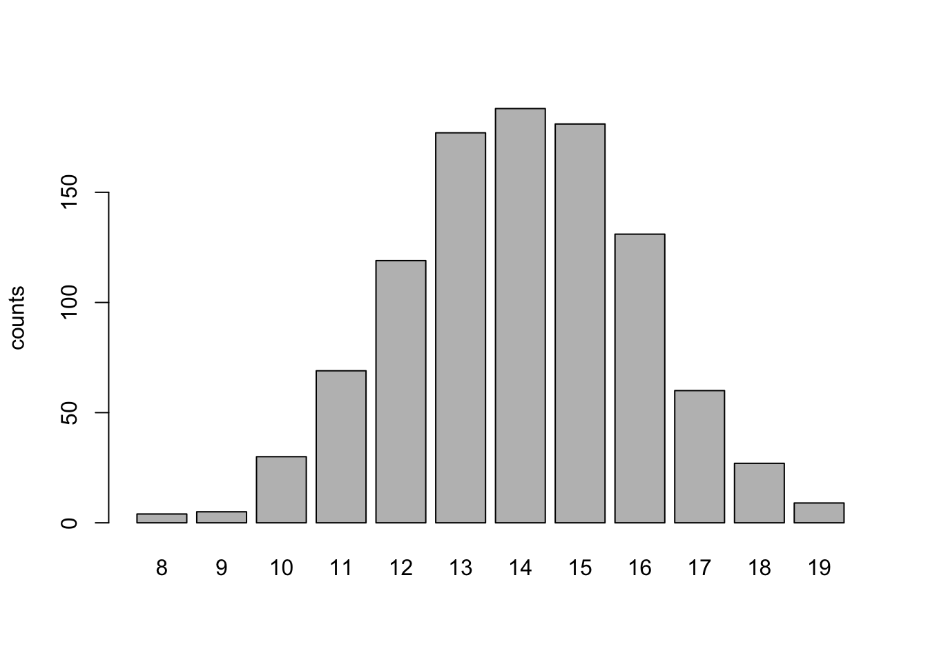
5.2.2.2 Density Functions: dbinom
The probability density function (PDF) of the binomial distribution is given by: \[f(x|n,p) = \Pr(X = x) = {n\choose x}p^x(1-p)^{n-x}\]
The function that computes this automatically is dbinom(). The d stands for “density” and the binom stands for “binomial”. Suppose we want to know the probability of getting 12 successes in 20 trials, we can calculate this easily with,
dbinom(x = 12, size = 20, p = 0.7)## [1] 0.1143967In fact, we can easily obtain and graph the probability of every possible outcome in this binomial distribution,
barplot(height = dbinom(0:20, size = 20, p = 0.7),
        names.arg = 0:20,
        main = "Binomial PDF", xlab = 'X', ylab = 'Probability')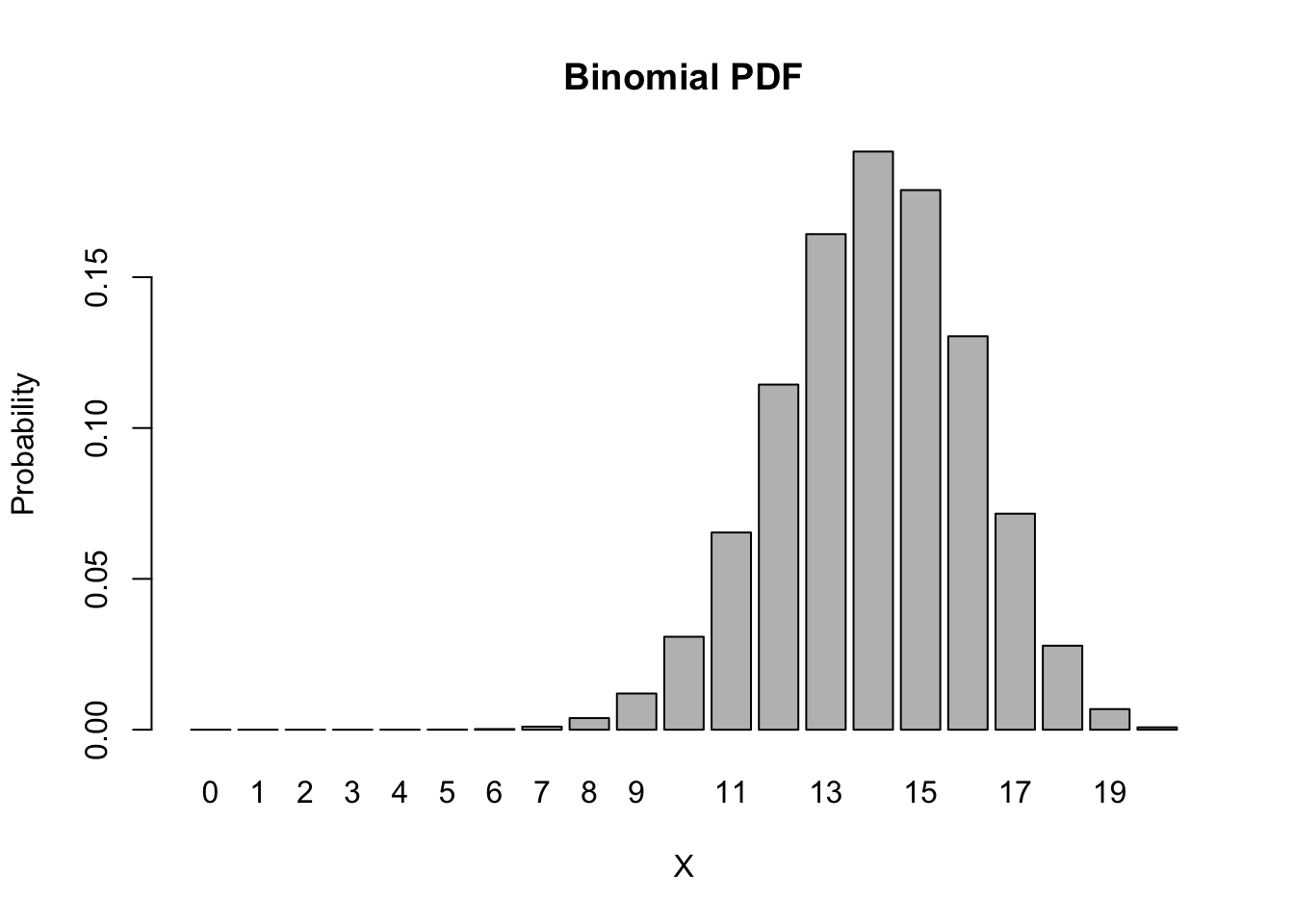
5.2.2.3 Cumulative Distribution Functions: pbinom
The cumulative distribution function (CDF) of the binomial distribution is given by: \[F(q|n,p) = \Pr(X \leq q) = \sum_{k=0}^q f(k|n,p)\]
Suppose we want to know the probability of getting at most 12 successes in 20 trials, we can obtain this easily with,
pbinom(q = 12, size = 20, p = 0.7)## [1] 0.2277282In fact, we can easily obtain and graph the entire CDF,
barplot(height = pbinom(0:20, size = 20, p = 0.7),
        names.arg = 0:20,
        main = "Binomial CDF", xlab = 'X', ylab = 'Probability')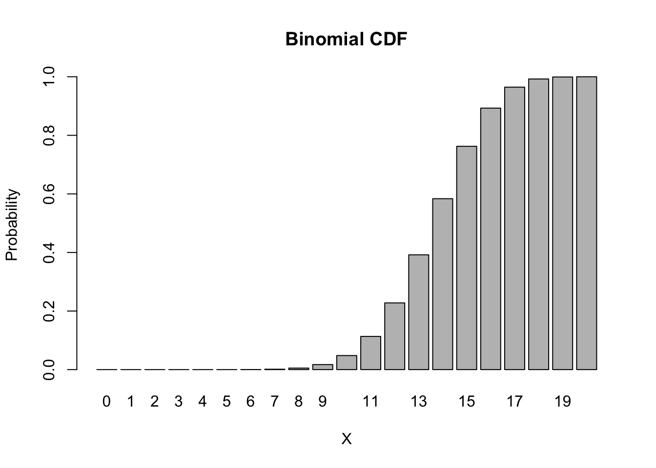
We can illustrate the relationship between the PDF and the CDF in the following plot,
par(mfrow = c(1,2))
barplot(height = dbinom(0:20, size = 20, p = 0.7),
names.arg = 0:20,
ylim = c(0,1),
main = "Binomial PDF", xlab = 'X', ylab = 'Probability',
col = c(rep("blue", 15), rep("gray", 8)))
barplot(height = pbinom(0:20, size = 20, p = 0.7),
names.arg = 0:20,
ylim = c(0,1),
main = "Binomial CDF", xlab = 'X', ylab = 'Probability',
col = c(rep("gray", 14), "blue", rep("gray", 6)))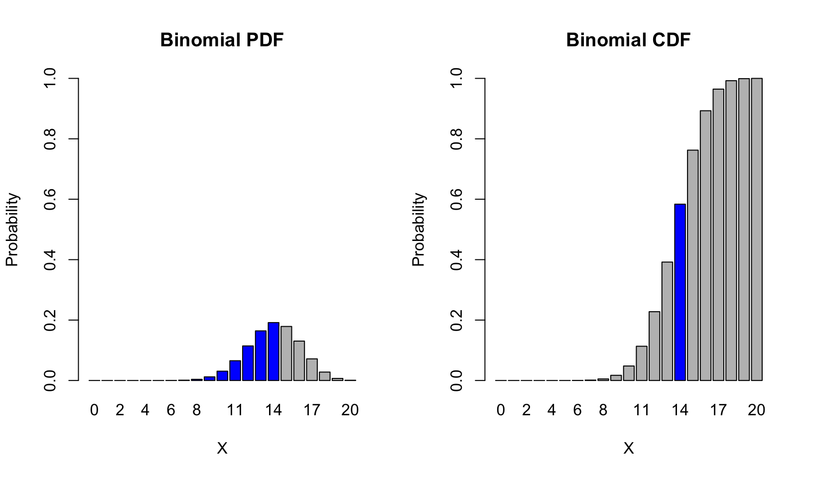 Notice that the value of the CDF at \(X = 14\) corresponds to the sum of the PDF from \(X = 0\) to \(X = 14\).
Properties of Distributions
Note that the sum of the densities is,
sum(dbinom(0:20, size = 20, p = 0.7))## [1] 1And we can obtain the expectation of this binomial distribution, using the general definition: \(\text{E}(X)=\sum{x_i \cdot P(X=x_i)}\)
sum(0:20 * dbinom(0:20, size = 20, p = 0.7))## [1] 14Note that this is also what we get using the specific formula for the expectation of a binomial: \(\text{E}(X) = np = 20 \cdot 0.7\).
The variance can be calculated using the general form: \(\text{Var}(X)=\sum{(x_i-\text{E}(X))^2 \cdot P(X=x_i)}\)
sum((0:20 - 20 * 0.7)^2 * dbinom(0:20, size = 20, p = 0.7))## [1] 4.2Which is equal to specific formula for the variance of a binomial: \(\text{Var}(X) = np(1-p) = 20 \times 0.7 \times 0.3\).
Exercises
Calculate the sum of 20 draws from a Bernoulli distribution with probability \(p = 0.9\), and report the result.
Obtain a vector of 1000 draws from the Binomial(n = 20, p = 0.7) distribution and compute the sample mean and sample variance. Do they agree with our predictions?
5.2.3 The Poisson Distribution
The Poisson distribution is a discrete distribution which was designed to count the number of events that occur in a particular time interval. A common (approximate) example is counting the number of customers who enter a bank in a particular hour. We traditionally call the expected number of occurrences \(\lambda\) or lambda.
Poisson vs. binomial: The key difference between the Poisson and the binomial is that for the binomial, the total number of trials in the sample is fixed, while for the Poisson, the total number of events in the interval is not fixed. That said, the binomial distribution begins to look a lot like the Poisson distribution when the number of trials grows large, and the probability of success is small.
5.2.3.1 Random Samples: rpois
As with the binomial, we can easily sample from the Poisson using the rpois() function, which now take takes two arguments:
n: how many outcomes we want to samplelambda: the expected number of events per interval
rpois(n = 10, lambda = 14)## [1] 12 14 18 13 9 13 10 17 20 8We can also plot a much larger sample of outcomes from this lambda = 14 Poisson distribution,
data = rpois(n = 1000, lambda = 14)
barplot(table(data))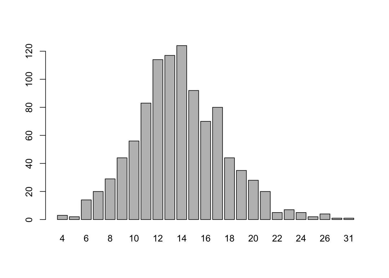
5.2.3.2 Density Functions: dpois
The probability density function (PDF) of the Poisson distribution is given by: \[f(x|\lambda) = \Pr(X = x) = \frac{\lambda^x e^{-x}}{x!}\] where \(e\) is equal to 2.7182818 and \(!\) is the factorial operator.
The function that computes this automatically is dpois(). The d stands for “density” and the pois stands for “Poisson”. Suppose we want to know the probability of getting 12 occurrences, we can get this easily with,
dpois(x = 12, lambda = 14)## [1] 0.09841849As before, we can easily obtain and graph the main part of the distribution,
barplot(height = dpois(0:30, lambda = 14),
        names.arg = 0:30,
        main = "Poisson PDF", xlab = 'X', ylab = 'Probability')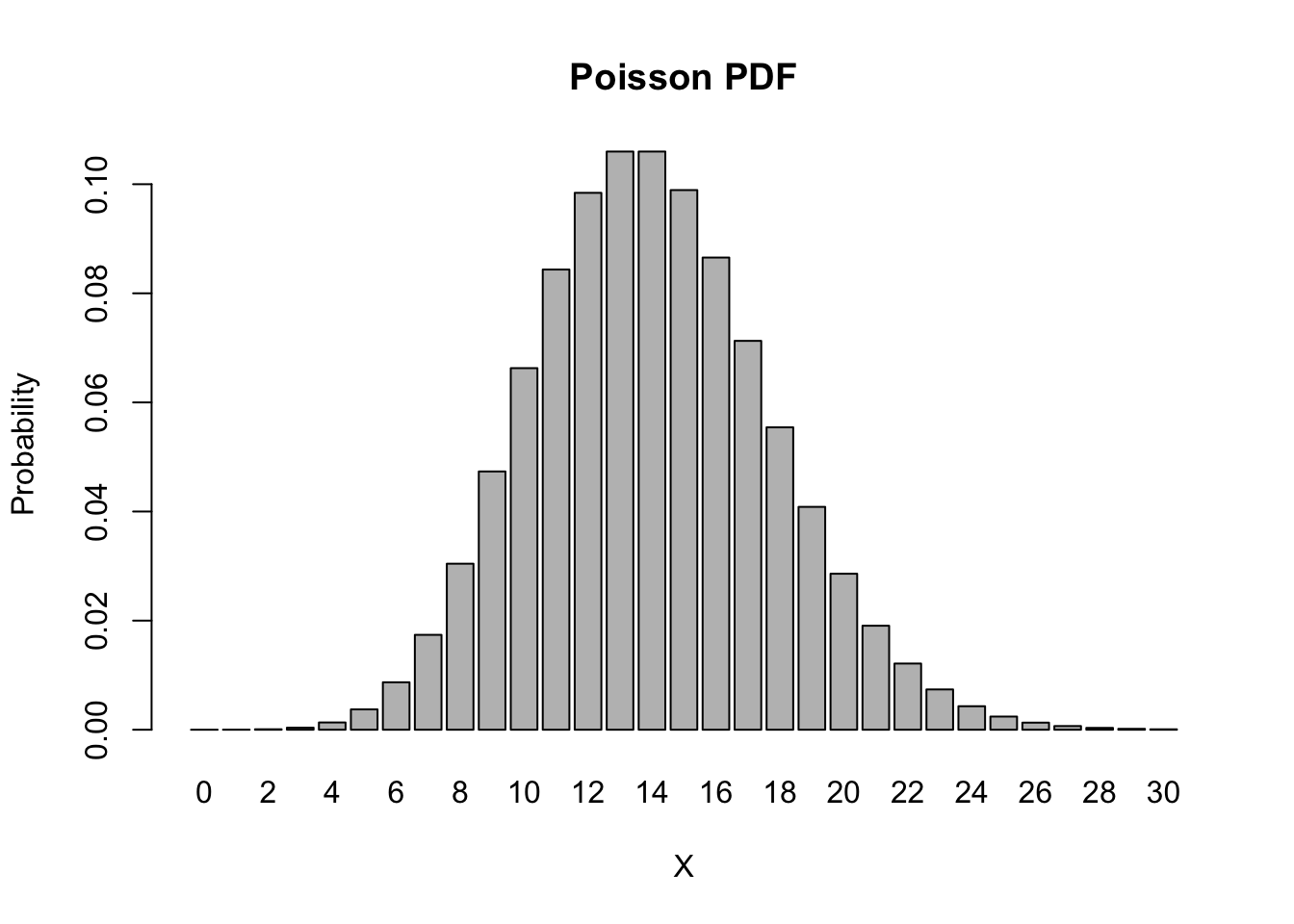
Note that this looks very much like the shape of the binomial distribution from the previous example. This is no coincidence, since the binomial(20, 0.7) and the Poisson(14) distributions are closely related (note that \(20 \cdot 0.7 = 14\)).
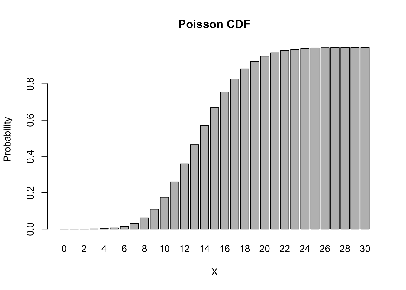
5.2.3.3 Cumulative Distribution Functions: ppois
The cumulative distribution function (CDF) of the Poisson distribution is given by: \[F(q|\lambda) = \Pr(X \leq q) = \sum_{k=0}^q f(k|\lambda)\]
Suppose we want to know the probability of getting at most 12 occurrences, we can get this easily with,
ppois(q = 12, lambda = 14)## [1] 0.3584584As before, we can easily obtain and graph the main part of the CDF,
barplot(height = ppois(0:30, lambda = 14),
        names.arg = 0:30,
        main = "Poisson CDF", xlab = 'X', ylab = 'Probability')