7.2 Checking Model Assumptions

The term “model diagnostics” refers to the plots and statistical tests that are used to evaluate both the assumptions and fit of a linear model. We will focus on some of these plots here. In R, there is an easy way to generate the most commonly used residual diagnostic plots:

par(mfrow=c(2,2))
plot(lin.model, pch = 16, col = "blue")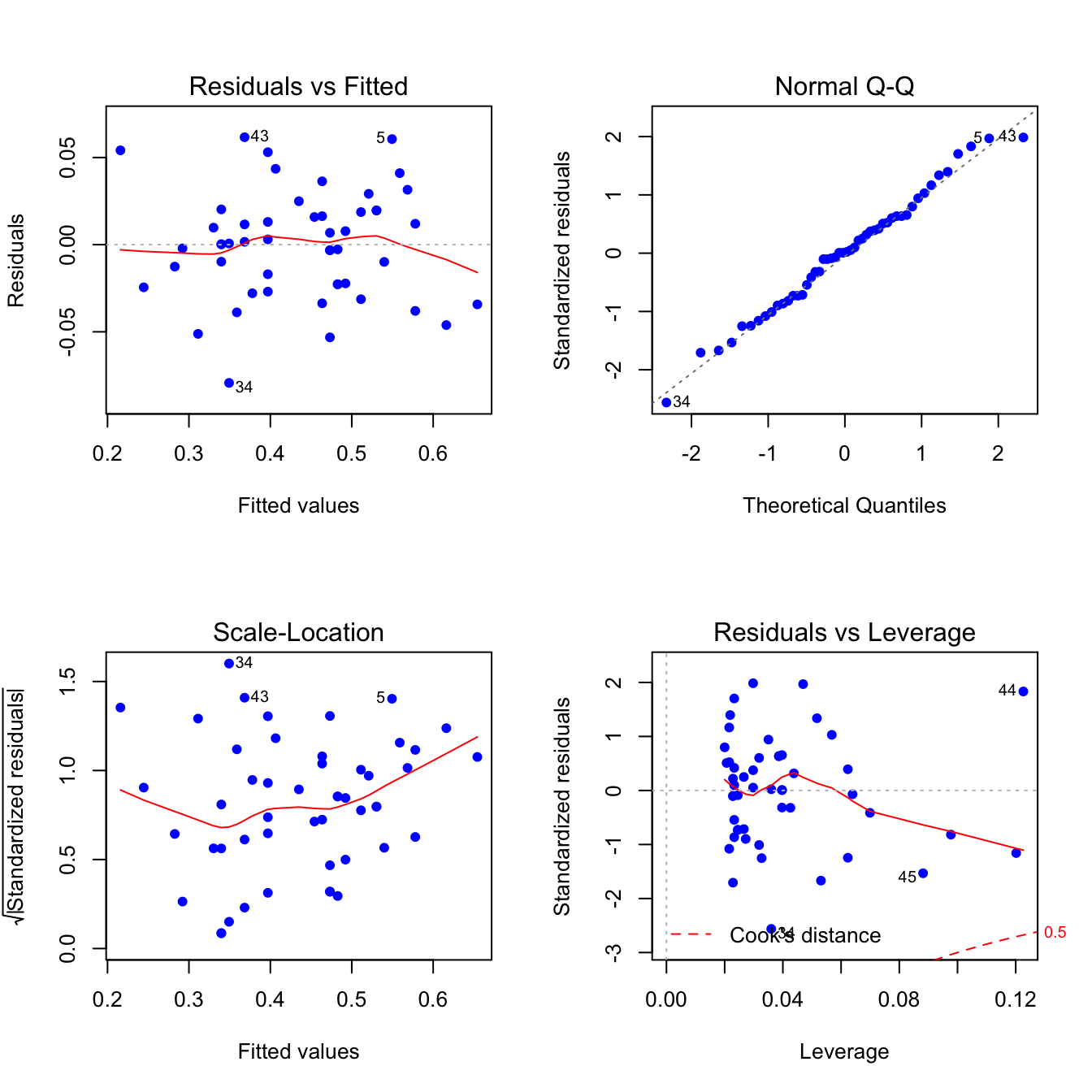

The output provides a lot of information (some of which we do not cover in this course).

The the first two plots we are familiar with: a scatterplot of the residuals vs. the fitted values \(\widehat{Y}_i\), and a QQ plot of the residuals agains the Normal quantiles. To make sure we understand these, we are going to build them up directly using the elements of the lin.model object.

We’ll start with the first plot: residuals vs. fitted values. This is used to check the assumptions for linearity and homoscedasticity. We can construct it directly from the components of the lin.model object:

plot(lin.model$residuals ~ lin.model$fitted.values,
     main = "Residual plot", 
     xlab = "Fitted Value", ylab = "Residual",
     pch = 16, col = "blue")
abline(h = 0, col = "red")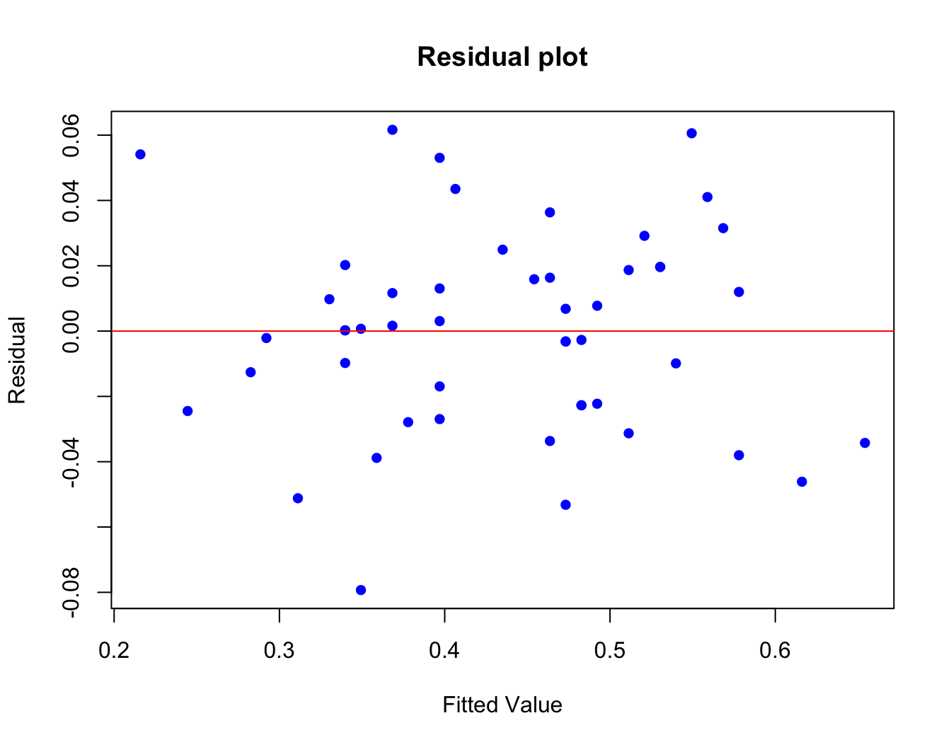

A “good” residual plot should have no noticeable patterns.

• What do you see here? Any cause for concern?

The second plot is a QQ-plot, used to check the assumption that the residuals are normally distributed: \(\epsilon_i \sim \mathcal{N}(0, \sigma^2)\). Remember that R function qqnorm compares the quantiles of the observed data (here our residuals) to the theoretical quantiles of the standard normal. So, we can easily construct this directly from the components of the lin.model object also:

qqnorm(lin.model$residuals,
       main = "Residual QQ plot",
       xlab = "Standard normal", ylab = "Residuals",
       pch = 16, col = "blue")
qqline(lin.model$residuals, col = "red")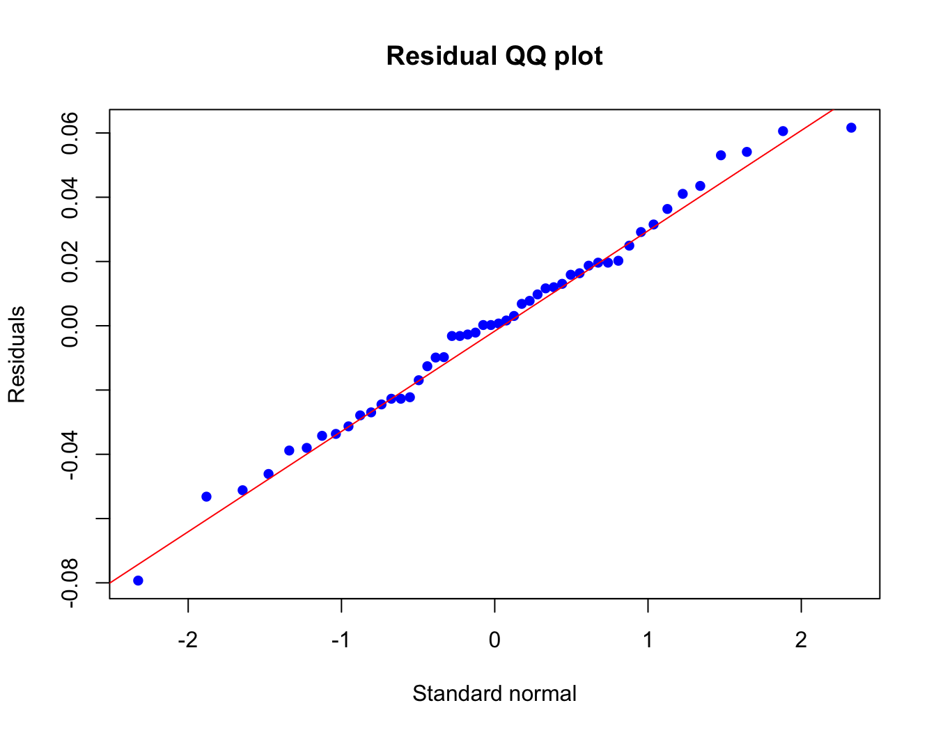

• What do you think? Do the residuals appear to be Normally distributed?

Having reviewed the regression output to verify that the assumptions needed for statistical inference are met, we can go on now to calculate and interpret Confidence Intervals and Hypothesis Tests.